Recently I played a bit with Robin Hood hashing, a variant of open addressing hash table. Open addressing means we store all data (key-value pairs) in one big array, no linked lists involved. To find a value by key we calculate hash for the key, map it onto the array index range, and from this initial position we start to wander. In the simplest case called Linear Probing we just walk right from the initial position until we find our key or an empty slot which means this key is absent from the table. If we want to add a new key-value pair we find the initial position similarly and walk right until an empty slot is found, here the key-value pair gets stored. Robin Hood hashing is usually described as follows. It's like linear probing, to add a key we walk right from its initial position (determined by key's hash) but during the walk we look at hash values of the keys stored in the table and if we find a "rich guy", a key whose Distance from Initial Bucket (DIB) a.k.a. Path from Starting Location (PSL) a.k.a. Probe Count is less than the distance we've just walked searching, then we swap our new key-value pair with this rich guy and continue the process of walking right with the intention to find a place for this guy we just robbed, using the same technique. This approach decreases number of "poors", i.e. keys living too far from their initial positions and hence requiring a lot of time to find them.

When our array is large and keys are scarce, and a good hashing function distributed them evenly so that each key lives where its hash suggests (i.e. at its initial position) then everything is trivial and there's no difference between linear probing and Robin Hood. Interesting things start to happen when several keys have the same initial position (due to hash collisions), and this starts to happen very quickly - see the Birthday Problem. Clusters start to appear - long runs of consecutive non-empty array slots. For the sake of simplicity let's take somewhat exaggerated and unrealistic case that however allows to get a good intuition of what's happening. Imagine that when mapping hashes to array index space 200 keys landed onto [0..100] interval while none landed onto [100..200]. Then in the case of linear probing it will look like this:

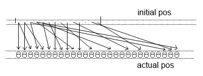
Many keys got lucky to land and stay on their initial positions, but there are also ones that landed very far from their initial buckets, we need to walk through the whole cluster to find them.

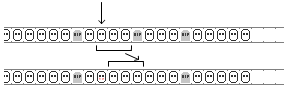
In the case of Robin Hood hashing it will look like this:

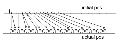
There are very few riches who remained their initial position. But there are also no very poor guys who require a walk through whole cluster to be found, we need to walk half the cluster at worst. It means the worst case became twice shorter and the average walk length got 25% shorter. Also here we can see the main property of Robin Hood hash table which is not obvious from its usual descriptions: all keys in the array are sorted by their initial positions. Because during insertions Robin Hood always favors the poor, the keys with longer distances from their initial buckets, which means a key with lower initial position will take the place of a key with higher initial position, moving it to the right. This understanding allows us to make an important optimisation: when we rob a rich guy making him search for a new place to live, all the ones to the right already have higher (or equal) initial positions, so we don't have to compute and compare them all when walking right, we can just shift right the whole part of cluster from this position to its end. Same result, less work. Another important optimisation: when we search for a key we don't have to walk from its initial position to the end of whole cluster. When, during the walk, we find a key whose initial position is greater than the one we're looking for, it means our key is not present in the table, we can give up the search. This makes searching for non-existing elements significantly faster than in linear probing.

Deletion. In the case of linear probing we find the key we want to delete and move to its slot the last value from the cluster, making it shorter.

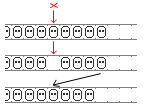
In the case of Robin Hood hashing we act differently: we mark the slot as deleted, leaving a tombstone that says "Mr. X lived here, his hash value was H".

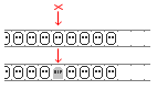
This is done to preserve the sorting of keys' starting positions. If we leave the deleted slot empty then when inserting some other key it may occupy this slot even if its initial position is greater than initial position of some key to the right of it, making that key impossible to be found. We also cannot move a key from the end of cluster to the deleted slot, this will break the sorting again. What we can do however is shift left the whole part of cluster from the deleted slot to the end of cluster. This is called "backward shift deletion" and some people called it an optimisation, because it reduces mean PSL and hence makes the search for keys faster. But the people who offered it did not bother to measure actual times. In reality it's not an optimisation, it makes things worse and slower. First, because the shifting takes significant time. And second, it makes insertion much slower. Because when we insert a key we shift right not the whole cluster but only a part till the first tombstone.

From insertion's point of view each deleted element divides the cluster in two parts, making it effectively twice shorter, reducing amount of data to be shifted when inserting. So tombstones make both insertion and deletion much faster than the backward shifting "optimisation". Of course, it's really a trade off between search speed and insertion & deletion speed, so the right choice depends on which operation is more important to you.

After making my own implementation (in D) I started testing it with random values of different types and discovered that when the key type is string my hash table works abysmally slow. My first guess was that hash function for strings was slow or maybe comparing string keys was slow. But no, that was not the case. On my random strings the hash function used by D for strings was not uniform enough, which caused clusters to appear and grow very quickly. And since complexity of one hash table operation is proportional to cluster size, time of n insertions grew as O(n²). For comparison I took an implementation of linear probing open addressing hash table from the vibe.d project. It showed absolutely the same problem: when keys were strings it was up to 50 times slower than D's built-in associative arrays which are hash tables with separate chaining (i.e. linked lists for each bucket). To fight this problem I added to my Robin Hood hashes monitoring of maximum cluster size so that when it exceeds some threshold the table grows even if its load factor is not very high yet. Of course we can't do it too often, or the table will eat all our RAM, so another parameter limits its growth so that the load factor doesn't fall below certain threshold when table grows.

Benchmark results turned out not very conclusive. In some cases one hash table is better, in some - another. Here's a table with times in milliseconds. Four implementations were measured: D's associative arrays (chaining based hash table), linear probing from vibe.d and two Robin Hood hashes, one where hashes are stored separately from the key-value pairs and one where they are stored together. Turns out in most cases it's better to store hashes separately.

For each combination of key-value types following operations were benchmarked:

• add_remove: a list of operations was generated consisting of n1 insertions, n2 deletions, n3 insertions, n4 deletions etc. of random values where n1,n2,... are also random numbers, total of 400 000 operations. Then all 4 hash table implementations executed this same list of operations.
• make_histo: for an array of 10 000 000 random values a histogram was calculated, i.e. counts of occurences for each value. So just insertions and updates. Again, one same input array for all hash table implementations. Value type is int.
• read_histo: for the same array of 10 000 000 keys, values (counts) from the histogram created by previous task were read for a simple operation, so this test is for lookups.

tags: programming